Final Project: Ship Detection with Random Forest and Artificial Neural Network

Alex Akin

Department of Atmospheric and Oceanic Sciences, UCLA

AOS C111: Introduction to Machine Learning for the Physical Sciences

Dr. Alexander Lozinski

December 8, 2023

Introduction

Remote sensing from space began in earnest with the launch of Landsat 1, the first Earth observation satellite, by NASA in 1972 [See Tatem et al. (2008) ¹ for further reading on the history of remote sensing]. The field has grown rapidly in recent years. Now, publicly-traded companies like Planet Labs are able to image the entire land surface of the Earth daily at unprecedented spatial scales, leading to a massive increase in the amount of data available. Planet maintains an image archive of 50 petabytes and operates 200 satellites, some having up to 50cm resolution. The amount of satellite imagery collected by Earth observation satellites is presently too large for careful human review.

Machine learning was first defined by Arthur Samuel in 1959, and closely related fields such as artificial intelligence and computer vision have evolved in tandem with it. The rapid growth of these fields has taken the world by storm in the past decade. They have numerous applications, from large language models to self-driving cars. Machine learning models can also be a helpful tool to apply in order to classify satellite images into useful categories, and this is the topic I seek to explore in this paper.

Data

Journalists at leading newspapers use Planet Labs imagery to provide a birds-eye view of many current events. For example, The New York Times Visual Investigations team found a Planet image of a cargo ship called Galaxy Leader that was anchored offshore before being hijacked off the coast of Yemen:

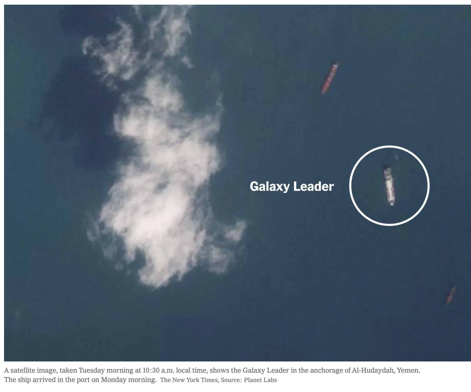
Inspired by the idea of identifying ships from satellite data, I obtained a dataset with the title Ships in Satellite Imagery from the data science platform Kaggle. The data was posted by the user rhammell, who shared 4000 80x80 RGB images “extracted from Planet satellite imagery over the San Francisco Bay and San Pedro Bay areas of California.” These are some of the busiest port areas in California for container shipping, being located in the state’s two main metropolitan areas: the Bay Area and Los Angeles. The ports of Los Angeles and Long Beach in particular are the busiest container shipping locations in the Western Hemisphere. Ship detection could potentially be a useful tool as a ground truth method for analyzing the number of ships offshore shipping ports. This could be relevant to understanding supply chains and industries such as logistics.

Of these 4000 images, 1000 were labeled as ‘ship’ and 3000 as ‘no-ship’. The particulars of each class are described below by the curator of the data set:

‘ship’: Images in this class are centered on the body of a single ship. Ships of different sizes, orientations, and atmospheric collection conditions are included.

‘no-ship’: A third of these are a random sampling of different land cover features - water, vegetation, bare earth, buildings, etc. - that do not include any portion of a ship. The next third are “partial ships” that contain only a portion of a ship, but not enough to meet the full definition of the “ship” class. The last third are images that have previously been mislabeled by machine learning models, typically caused by bright pixels or strong linear features.

In other words, the author intentionally constructed this data set to give machine learning engineers an interesting challenge due to the diversity in the conditions and characteristics of the imagery.

The images can be loaded in as an array of shape 4000x80x80x3, and flattened to 4000 images of 19200 values. This comes out to 73.24 megabytes, which is a manageable size to train machine learning models in the Google Colab environment.

To illustrate the differences between these two classes of imagery, I plotted their average red, green, and blue values (recall that RGB values range from 0-255 and signify the intensity of each color) over an 80x80 grid. I also added the average value of every 20x20 square to make the trends more clear.

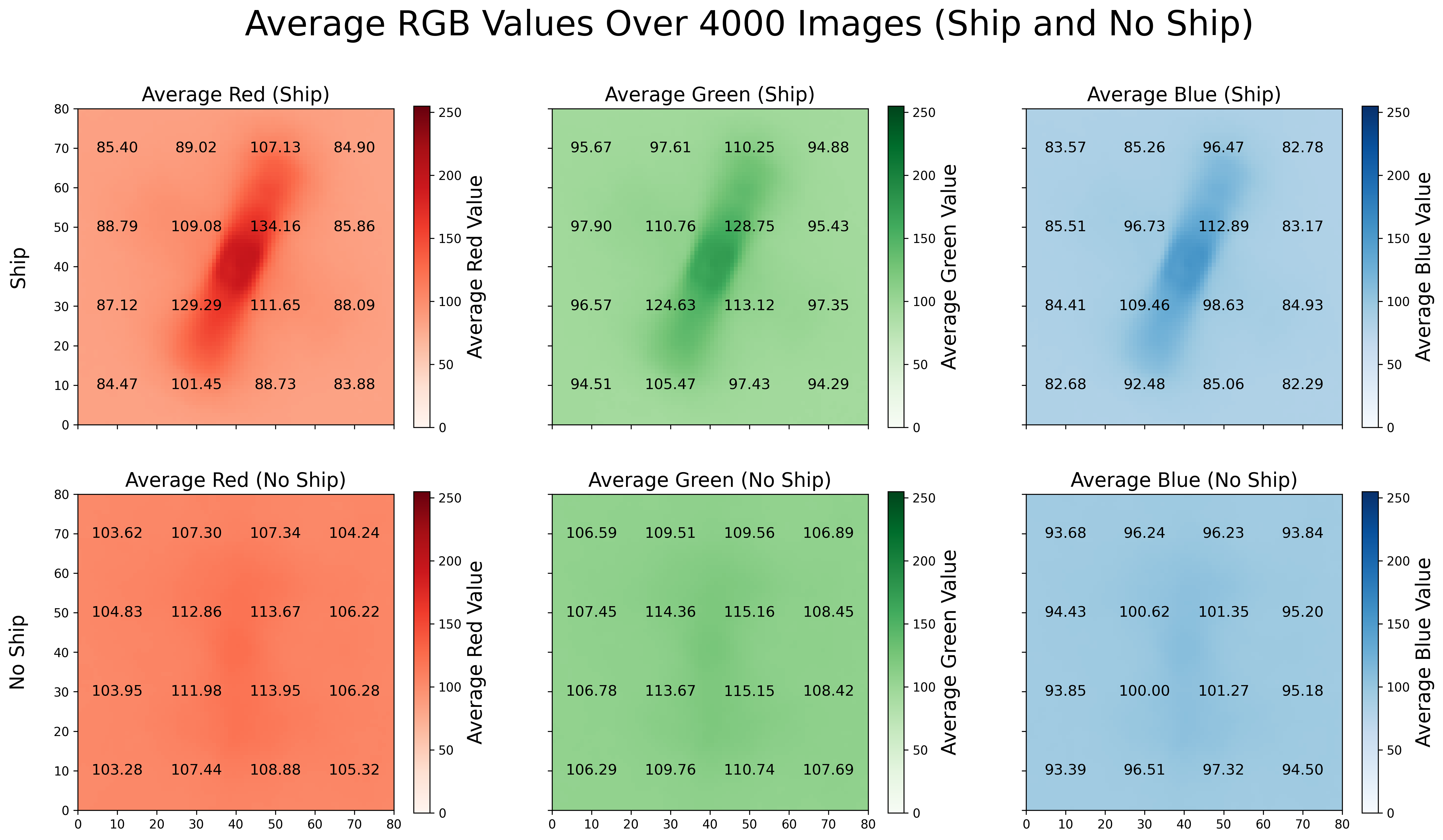
Figure 1: Average RGB values

We can clearly see the distinction between the ‘ship and ‘no-ship’ classes in all three channels: note the considerably darker shading in the middle of the images for the first row and the absence of that in the second row. In other words, the ‘ship’ class has higher values in the center of the image and lower values toward the edges, while ‘no-ship’ has much more uniform values.

Note that the average ship included in the ‘ship’ class is tilted at about a 20 degree angle to the right of the vertical, extends from 10 to 70 on the y-axis and 20 to 60 on the x-axis, and is about 10 pixels wide. Also, the center of the average ship has higher average RGB values than the bow or the stern, which tracks since not all the ships are oriented this way but are all centered in order to be included in the ‘ship’ class. In the ‘no-ship’ class, there is still a small increase of about 10 from the RGB values on the edge of the image to those at the center. This could be due to the inclusion of 1000 “partial ships” as a third of the 3000 image ‘no-ship’ class.

There are also eight scenes included in the data set, which are larger satellite images (thousands of pixels wide and tall) that capture large areas of the San Francisco and San Pedro Bays. I will use these, as intended by the author, as a way to visualize the performance of the model after it has been trained on the 4000 smaller images. This will be a qualitative assessment rather than a quantitative one.

Modeling

I used two different machine learning approaches: a random forest of decision trees and an artificial neural network to classify the images in the data set.

A random forest is an ensemble method that improves upon the performance of an individual decision tree. As my data set was labeled, this is considered supervised learning. Specifically, I selected a binary classification tree architecture, meaning that my decision trees returns either a 0 (‘no-ship’) or 1 (‘ship’). I built it using scikit-learn’s RandomForestClassifier implementation. I experimented with hyperparameters using RandomizedSearchCV, and landed on these: n_estimators=300, max_depth=25, min_samples_leaf=5 with class_weight='balanced'.

I used the keras interface of the TensorFlow library to construct my ANN. For my artificial neural network architecture, I chose a deep learning model with four hidden layers configured with ReLU activations:

model = models.Sequential([
    layers.InputLayer(input_shape=(flattened_images.shape[1],)), # Input layer
    layers.Dense(300, activation = 'relu'), # First hidden layer 
    layers.Dense(100, activation = 'relu'), # Second hidden layer
    layers.Dense(100, activation = 'relu'), # Third hidden layer
    layers.Dense(100, activation = 'relu'), # Fourth hidden layer
    layers.Dense(1, activation='sigmoid')  # Output layer for binary classification
])

I experimented with various architectures before arriving at this. The deep learning model performs decently well on the scenes as plotted in the Discussion section, but this architecture did not produce the highest accuracies on the actual training and test data when compared to simpler architectures. Compared to the random forest model, the artificial neural networks I experimented with took much longer to train and implement.

Results

I ran the random forest model, achieving a test accuracy of 96.50% and a training accuracy of 99.47%. Plotted below is the confusion matrix for the model alongside the feature importances on an 80x80 grid:

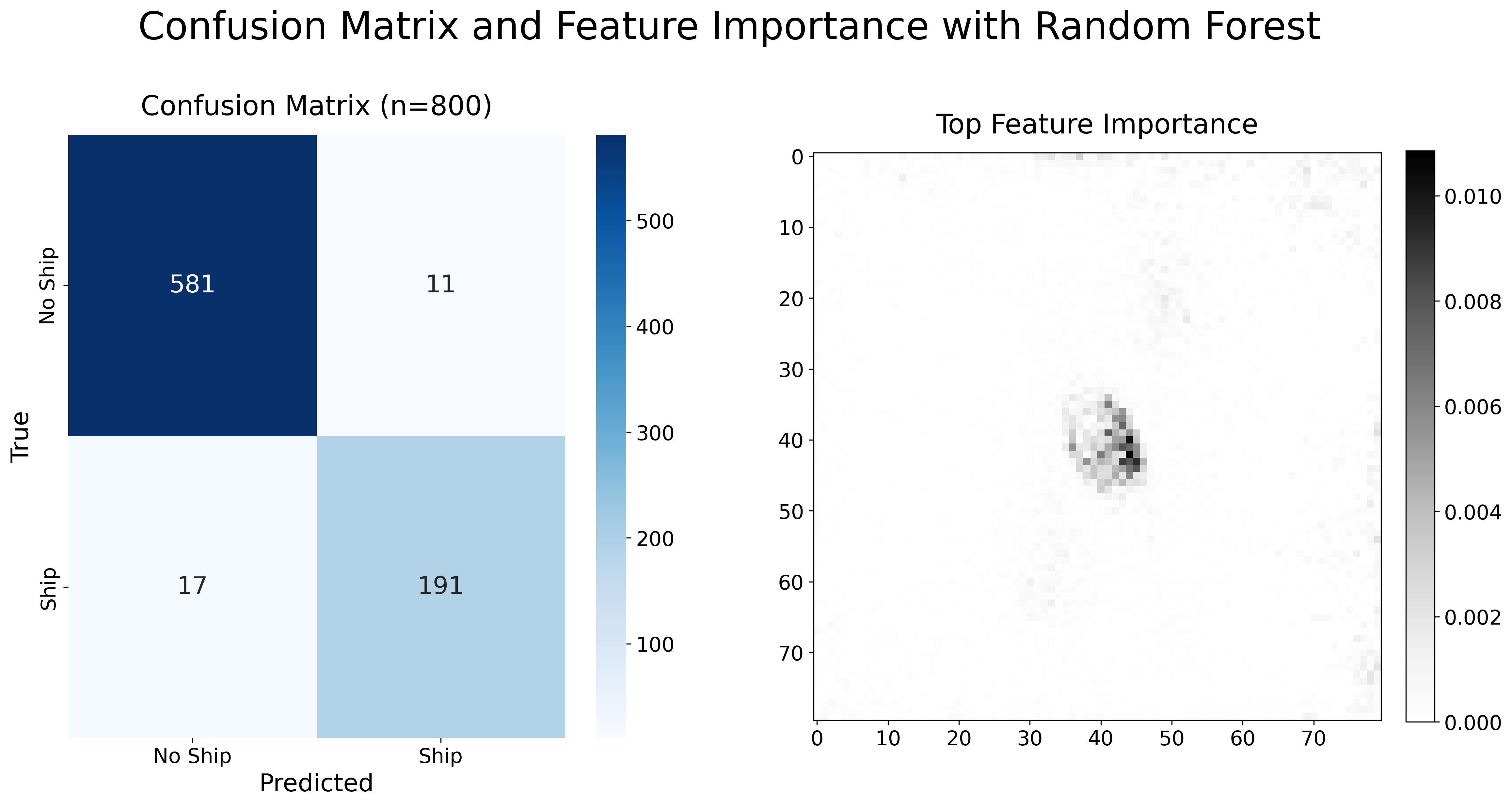
Figure 2: Confusion Matrix and Feature Importance for Random Forest

This model is predicting fewer false positives (11) than false negatives (17). Interestingly, the highest feature importances are all clustered at the center of the 80x80 grid, meaning that the pixels at the center of the images are most important and informative for making correct predictions. This confirms what we know about the labels: that the images in the ‘ships’ class “are centered on the body of a single ship”, which is what distinguishes them from the ‘no-ship’ class. Therefore, this plot of feature importance for my random forest model makes intuitive sense given the structure of the data set.

Below are the ROC and Precision-Recall curves, which are useful visualizations of the model’s performance:

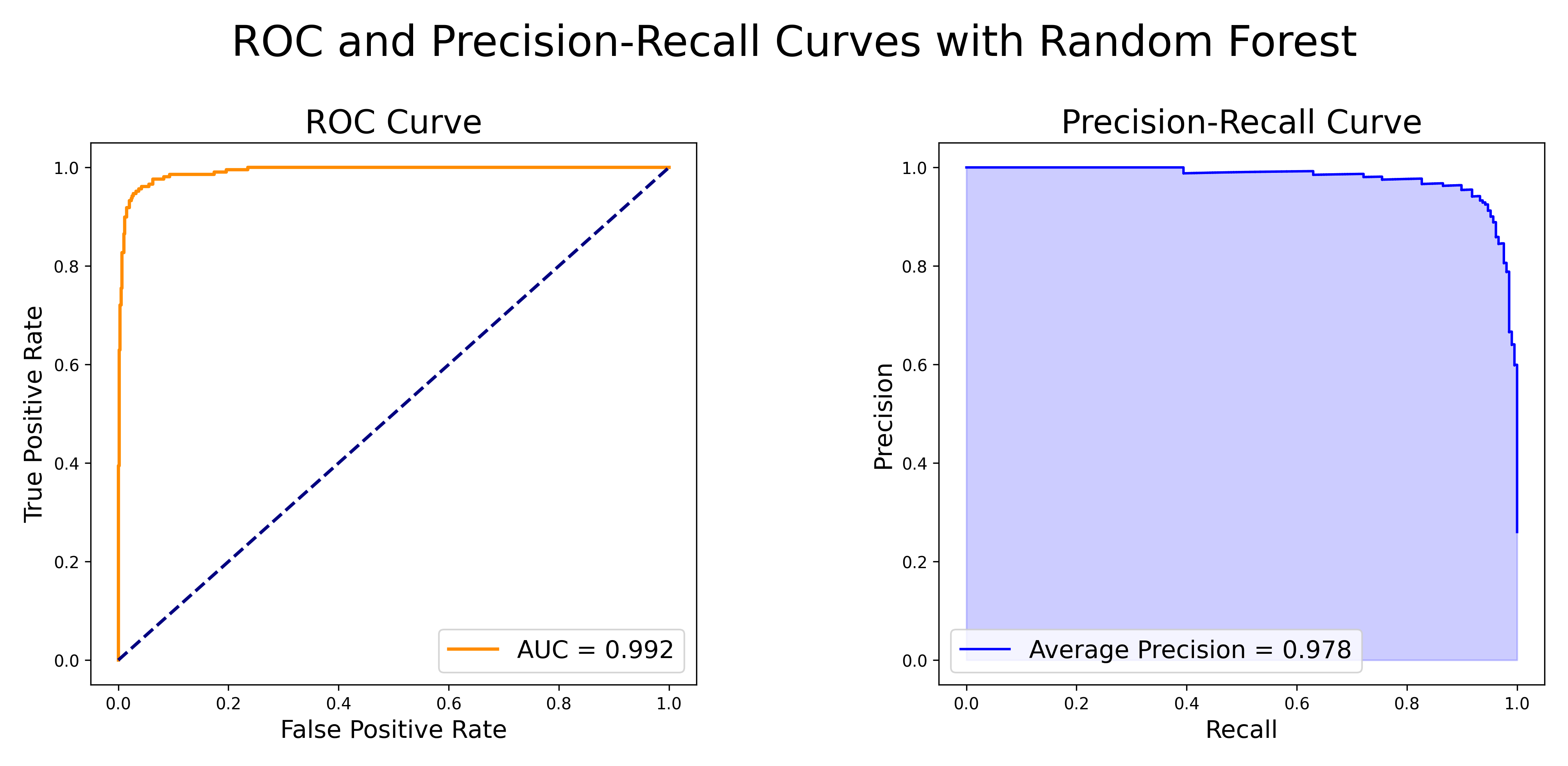
Figure 3: ROC and Precision-Recall Curves for Random Forest

On the left subplot, we see the ROC curve with a baseline classifer that performs no better than random chance plotted as y=x. On the right subplot, the Precision-Recall curve is plotted.

The values of the two evaluation metrics shown on the above plot of the ROC and Precision-Recall Curves, AUC (Area Under Curve) and AP (Average Precision), can range from 0 to 1. Values closer to 1 mean that the model is exhibiting excellent performance at the binary classification task. This is certainly the case here, as AUC=0.992 and AP=0.978.

The ANN achieved a test accuracy of 89.25% and a training accuracy of 86.29%. Below, the confusion matrix is plotted with the ROC and Precision-Recall curves:

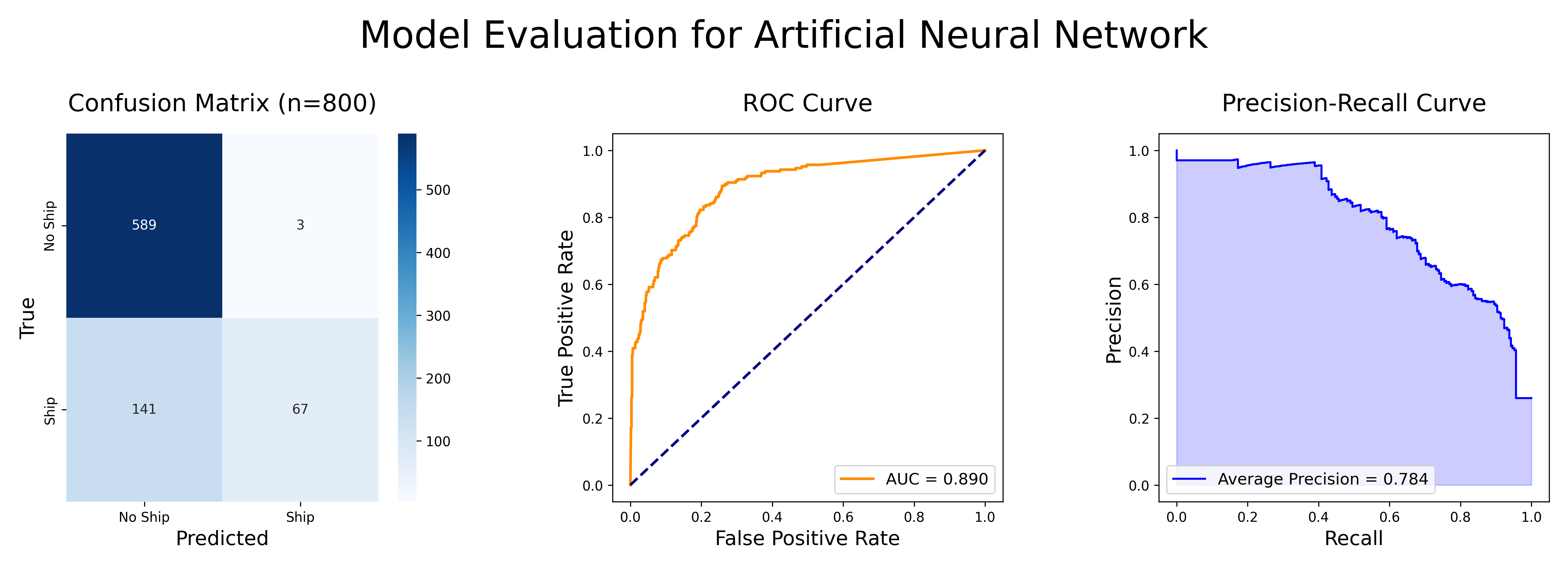
Figure 4: Model Evaluation for Artificial Neural Network

This model has a high precision but low recall; only 3 false positives but 141 false negatives. This is less false positives than the random forest model, but many more false negatives. One can also see that the ANN performs much worse on the ROC and Precision-Recall curves compared to the random forest.

Discussion

Finally, I used my model to classify ships with seven of the provided scenes (I left out the 8th scene, ‘sfbay_1’, because it had 4 channels rather than matching the 3 channels of the RGB training data). These scenes were included as a way to visualize the performance of the model as it is applied across a satellite image of a larger area. I used a sliding windows approach to accomplish this. I divided the scene up into 80x80 overlapping images (with a step size of 10) and applied the model to each image, iterating over the entire scene. Then, I plotted bounding boxes around each ‘ship’ as predicted by the model.

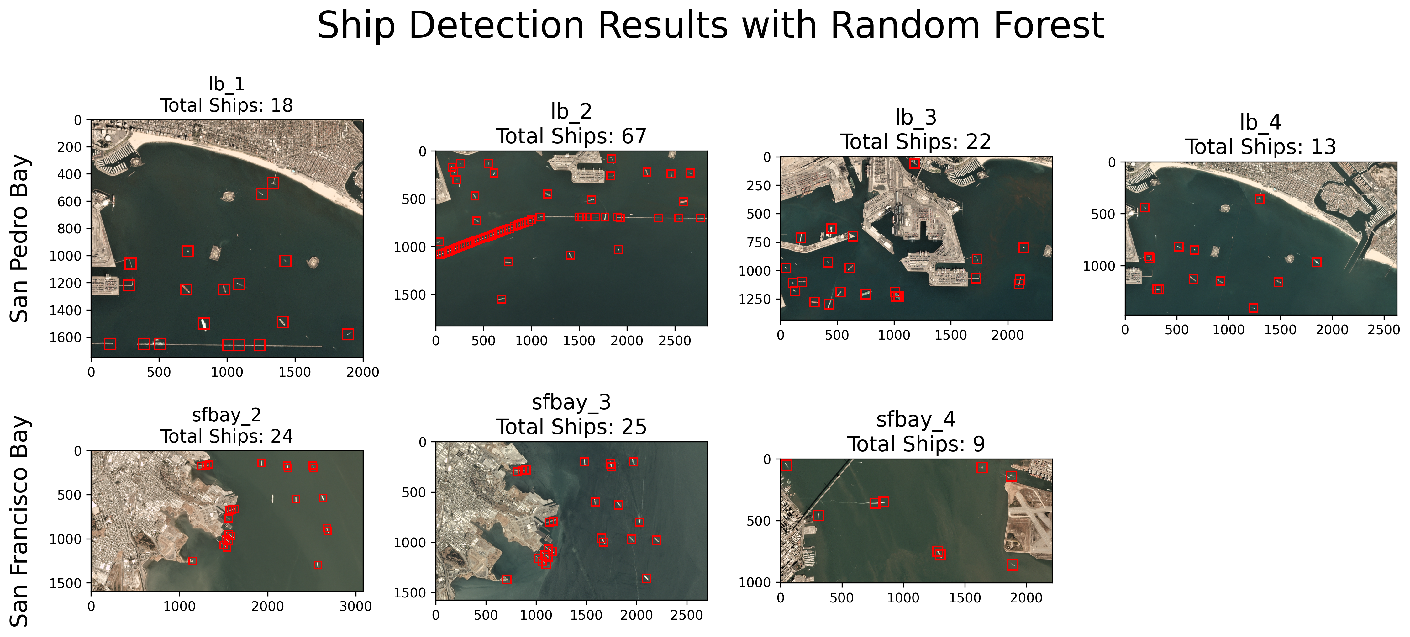
Figure 5: Ship Detection Results with Random Forest

We can see that the random forest is classifying most of the actual ships correctly, but is generalizing poorly to parts of the scene such as piers and breakwaters. For example, in ‘lb_2’, nearly the entire left side of the Long Beach breakwater is being classified as ships. This is interesting when you compare with the right side of the Long Beach breakwater, which is not being as aggressively predicted as being ships. The difference is that the left side is oriented at a roughly 30 degree angle from the horizontal, while the right side lays flat along the horizontal. Recall Figure 1 and one can note that the left side of the breakwater is oriented closer to the average ‘ship’ image.

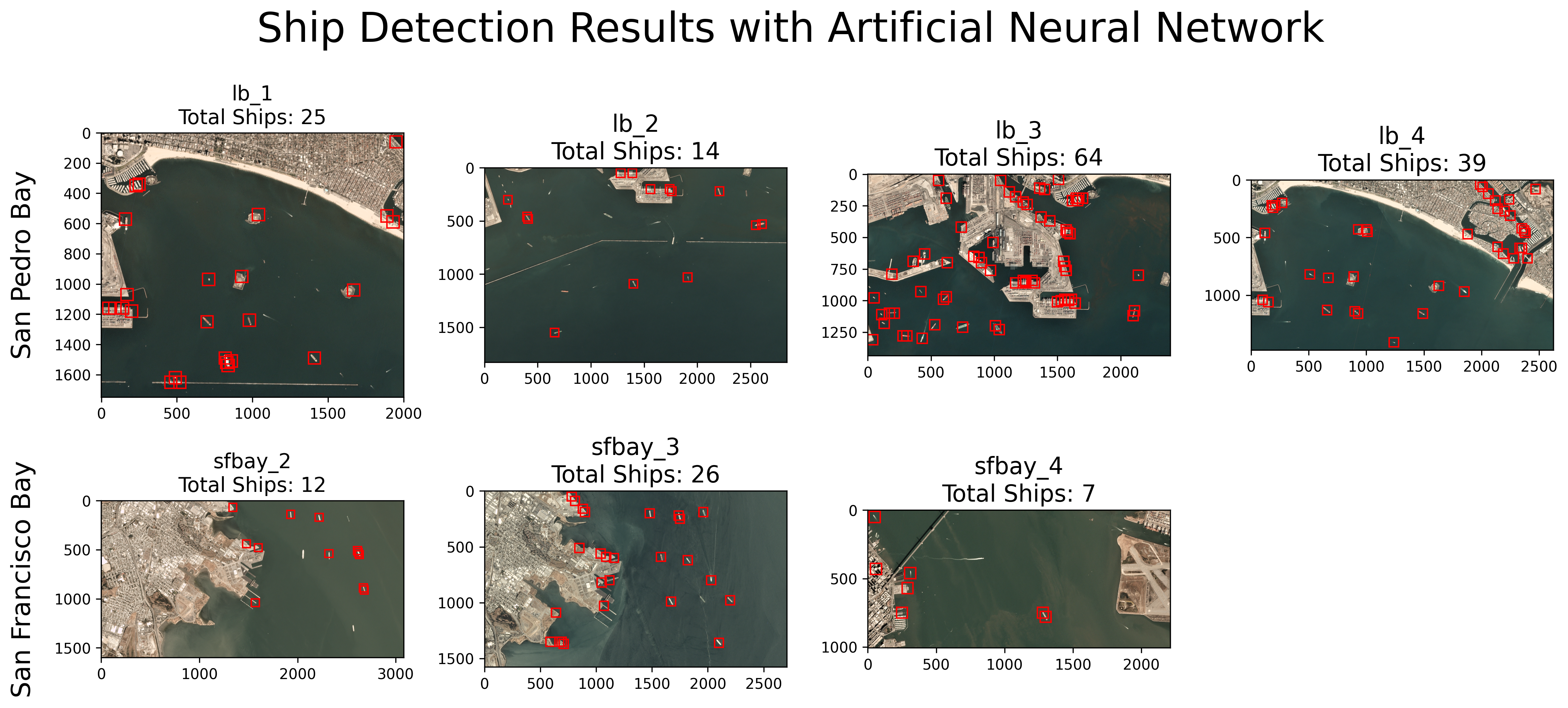
Figure 6: Ship Detection Results with Artificial Neural Network

In contrast with the random forest results, this artificial neural network doesn’t have a problem with breakwaters, which represent relatively “skinny” lines running across a given image. However, it has significant issues with coastal images. In Alamitos Bay in ‘lb_4’ (located in the upper right), one can visually see that there are many false positives along the water channel. The ANN also performs worse at classifying the actual ships when compared to the RF model.

Belgiu and Drăguţ (2016)² mention that random forests have been implemented successfully to classify satellite imagery sourced from both commercial and governmental programs, including NASA (MODIS, Landsat, and IKONOS), the European Space Agency (WorldView-2), and Planet Labs itself (RapidEye). These models were used to create maps of boreal forest habitats, tree biomass, canopy cover, and insect defoliation levels. Belgiu and Drăguţ note that random forest models “outperform decision tree classifiers (Ghimire et al., 2012, Gislason et al., 2006, Han et al., 2015)…and ANN classifiers (Chan and Paelinckx, 2008) in terms of classification accuracy.” This lines up with the performance of the models here, with the random forest outperforming the ANN.

Conclusion

We can see that each model has its own emergent strengths and weaknesses due to the fundamental differences in architecture between a random forest and a neural network. However, we can see that the random forest model clearly wins out, both when applied to the test data and over entire scenes; it correctly identified nearly all the actual ships. The high rate of false positives when generalizing the model to scenes presents a significant issue if one is aiming to apply a similar model to satellite imagery of various sizes. An improved model would need to be developed, perhaps requiring more computational resources and time. Convolutional neural networks could be an interesting architecture to implement in similar ship detection problems in the future. Additionally, obtaining a different data set with more images could be helpful. Future studies could also expand beyond binary classification to classify various types of ships and different classes of atmosphere, land, and ocean features.

References

1. Tatem, A. J., Goetz, S. J., & Hay, S. I. (2008). Fifty Years of Earth Observation Satellites: Views from above have lead to countless advances on the ground in both scientific knowledge and daily life. American Scientist, 96(5), 390–398. https://doi.org/10.1511/2008.74.390 ↩

2. Belgiu, Mariana, and Lucian Drăguţ. “Random Forest in Remote Sensing: A Review of Applications and Future Directions.” ISPRS Journal of Photogrammetry and Remote Sensing, vol. 114, Apr. 2016, pp. 24–31. ScienceDirect, https://doi.org/10.1016/j.isprsjprs.2016.01.011. ↩